What is Transient heat transfer?
The type of heat transfer in which, the temperature of the body changes with respect to time is known as transient heat transfer.
It is also known as the Unsteady-state heat transfer.
Therefore for transient heat transfer,
`\frac{dt}{\partial \tau }` ≠ 0
Where,
dt = Change in temperature
d𝜏 = Time interval
In transient heat conduction, the temperature and rate of heat flow at a point change continuously with respect to time.
In this article, we’re going to discuss:
- Transient heat transfer examples:
- Different cases of Transient heat transfer:
- Biot number:
- Methods to solve transient heat transfer:
Transient heat transfer examples:
In real conditions, the heat transfer mostly takes place in a transient way. Here are some examples of transient heat transfer.
- Heating or cooling of the IC engines.
- Heat transfer in buildings in day.
- Cooling or heating of foods.
- Heating of metal bar.
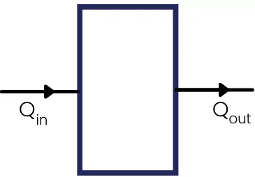
When the rate of heat energy entering into the body does not match with the rate of heat leaving the body, then the internal energy of the body increases or decreases, and therefore the temperature of the body increases with respect to time.
That is, `Q_{\text{in}}` ≠ `Q_{Out}`
`\Delta E` ≠ 0
`\frac{dt}{\partial \tau }` ≠ 0
Therefore this situation is known as Transient or Unsteady state heat transfer.
Different cases of Transient heat transfer:
Case 1:-
When one end of the object is subjected to a heat source and another end is in contact with a sink with no internal heat generation and If `Q_{\text{in}} > Q_{Out}`
Then heat gained by body is positive.
`\Delta E` = +ve
Hence `\frac{dt}{\partial \tau }` = +ve
Therefore it is the case of Transient heat transfer.
Case 2:-
When `Q_{\text{in}} < Q_{Out}`and `Q_{\text{generation}}=0`, then the energy of the body is lowered.
`\Delta E` = -ve
Hence `\frac{dt}{\partial \tau }` = -ve
It is also case of Transient heat transfer.
Case 3:-
When the object is completely surrounded by the source.
In this case `Q_{Out}`= 0 and `Q_{\text{in}}` = +ve
Therefore the internal energy of the object continuously increases.
`\Delta E` = +ve
Hence `\frac{dt}{\partial \tau }` = +ve
It is Transient heat transfer.
Example:- Heating of metal bar in the furnace.
Case 4:-
When the object is completely surrounded by the low-temperature sink.
In this case, heat is lost by the object.
Hence `Q_{\text{in}}` = 0 and `Q_{\text{out}}`
Therefore the internal energy of the object is continuously decreasing.
`\Delta E` = -ve
Hence `\frac{dt}{\partial \tau }` = -ve
In this case, the temperature of the body decreases with respect to time and it is also the case of transient heat transfer.
Biot number:
The biot number represents the distribution of temperature within the body.
Biot number is defined as the ratio of conductive resistance of the body to the convective resistance on the surface of the body.
Mathematically it is given by,
Bi = `\frac{\text{Internal conductive resistance}}{\text{External convective resistance}}`
Bi = `\frac{\frac{L_{C}}{K.A}}{\frac{1}{hA}}` = `\frac{hL_{C}}{K}`
Bi = `\frac{hL_{C}}{K}`
The lower value for the biot number indicates that the object has less conductive resistance in comparison with convective resistance therefore the value of the temperature gradient is less.
If the value of the Biot number is higher, then the object has comparatively higher conductive resistance in comparison with convective resistance, and in this case, the value of the temperature gradient is higher.
The following figure shows the temperature distribution in the body for both these conditions.
Methods to solve transient heat transfer:
1] Lumped system analysis:-
The lumped system analysis method is used when the value of the biot number is less than 0.1.
In this case, the conductive resistance of the object is considered negligible. It means that the material has very high thermal conductivity.
The temperature distribution in such conditions is considered uniform throughout the body (The temperature of the body is constant).
The relation for lumped capacity method is given by,
`\frac{t-t_{\infty}}{t_{1}-t_{\infty}}`= `e^-{\frac{h.A}{\rho .V.C}}` When Bi < 0.1
Where,
t = Temperature of object after of 𝜏
`t_{\infty}`=Atmospheric temperature
`t_{1}` = Initial temperatre of object at 𝜏=0
As = Surface area of object
ρ = Density of object
V = Volume of object
C = Specific heat of object
h = Convective heat transfer coefficient of medium
𝜏 = Time to reach temperature of object from initial temperature to final temperature
2] Heisler chart:-
Heisler chart is the graphical method to analyze transient heat conduction system
The Heisler chart method is used when 0.1 < Bi < 100
The Heisler chart is different for infinite long plane wall, cylinder, and sphere.
Read also: